Visual Multivariate Analysis with Parallel Coordinates Plot

1. Learning Outcome

In this hands-on exercise, we will learn how to make parallel coordinates plot.

2. Getting Started

2.1 Installing and loading the required libraries

Firstly, let’s install and load the required packages:

• tidyverse: an opinionated collection of R packages designed for data import, data wrangling and data exploration

• GGally: extends ‘ggplot2’ by adding several functions to reduce the complexity of combining geometric objects with transformed data.

• parallelPlot: Constructs a parallel coordinate plot for a data set with classes in last column.

pacman::p_load(tidyverse, GGally, parallelPlot)

2.2 Importing the data

We’ll use the data of World Happines 2018 report for this hands-on exercise. The original data is stored in an excel file, and it’s been converted to a csv file for easy importing.

Let’s start by importing the data.

wh  <- read_csv("../../Data/WHData-2018.csv")

The data contains 156 rows and 12 columns:

• 2 character variables:
  • Country
  • Region
• 10 numerical variables:
  • Happiness score
  • Whisker-high
  • Whisker-low
  • Dystopia
  • GDP per capita
  • Social support
  • Healthy life expectancy
  • Freedom to make life choices
  • Generosity
  • Perceptions of corruption

3. Plotting Static Parallel Coordinates Plot

n this section, we will learn how to plot static parallel coordinates plot by using ggparcoord() of GGally package.

3.1 Plotting a simple parallel coordinates

ggparcoord(data = wh, 
           columns = c(7:12))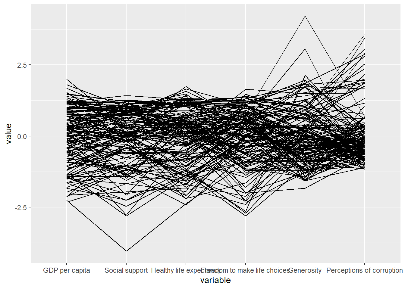

It’s quite obvious to see that there are some outliers in the following columns:

• Social support
• Freedom to make life choices
• Generosity
• Percveptions of corruption

3.2 Plotting a parallel coordinates with boxplot

However, it’s quite difficult understand the distribution of the columns. We can overcome this by adding boxplots.

ggparcoord(data = wh, 
           columns = c(7:12), 
           groupColumn = 2,
           scale = "uniminmax",
           alphaLines = 0.2,
           boxplot = TRUE, 
           title = "Parallel Coordinates Plot of World Happines Variables")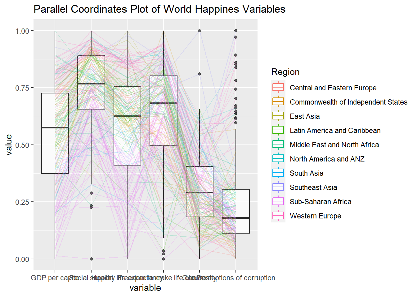

We can now make more statistical inference from the plot.

3.3 Parallel coordinates with facet

We can further break it down by facet to visualize the differences among different categories.

ggparcoord(data = wh, 
           columns = c(7:12), 
           groupColumn = 2,
           scale = "uniminmax",
           alphaLines = 0.2,
           boxplot = TRUE, 
           title = "Multiple Parallel Coordinates Plots of World Happines Variables by Region") +
  facet_wrap(~ Region)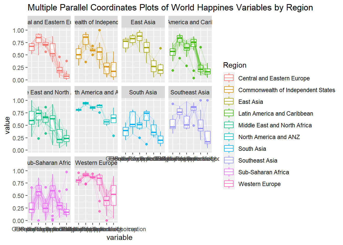

Now we have made the parallel coordinates plots for each region.

3.4 Rotating x-axis text label

Let’s now customize the plots a bit to make the x-axis labels easier to be read.

ggparcoord(data = wh, 
           columns = c(7:12), 
           groupColumn = 2,
           scale = "uniminmax",
           alphaLines = 0.2,
           boxplot = TRUE, 
           title = "Multiple Parallel Coordinates Plots of World Happines Variables by Region") +
  facet_wrap(~ Region) + 
  theme(axis.text.x = element_text(angle = 30))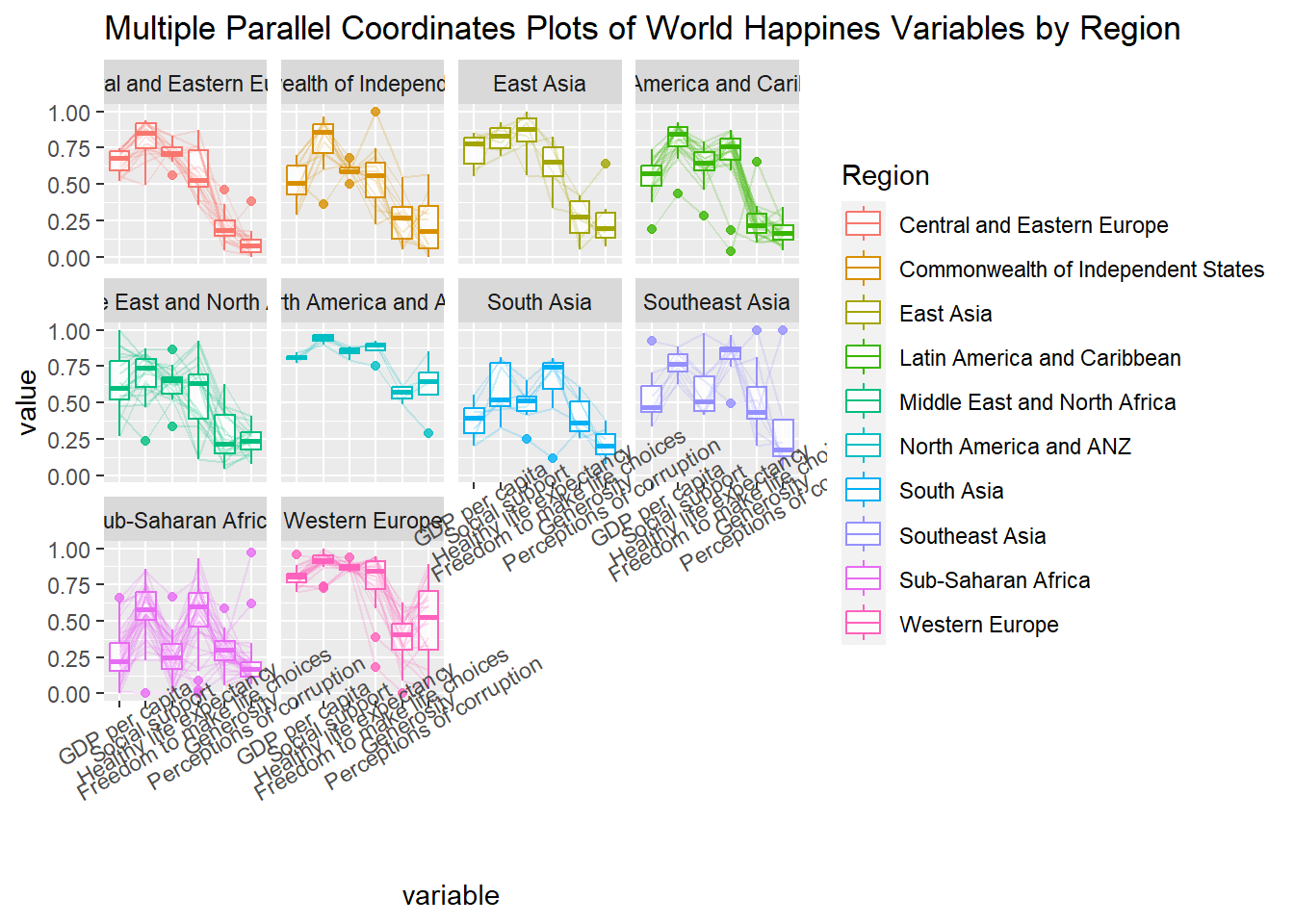

ggparcoord(data = wh, 
           columns = c(7:12), 
           groupColumn = 2,
           scale = "uniminmax",
           alphaLines = 0.2,
           boxplot = TRUE, 
           title = "Multiple Parallel Coordinates Plots of World Happines Variables by Region") +
  facet_wrap(~ Region) + 
  theme(axis.text.x = element_text(angle = 30, hjust=1))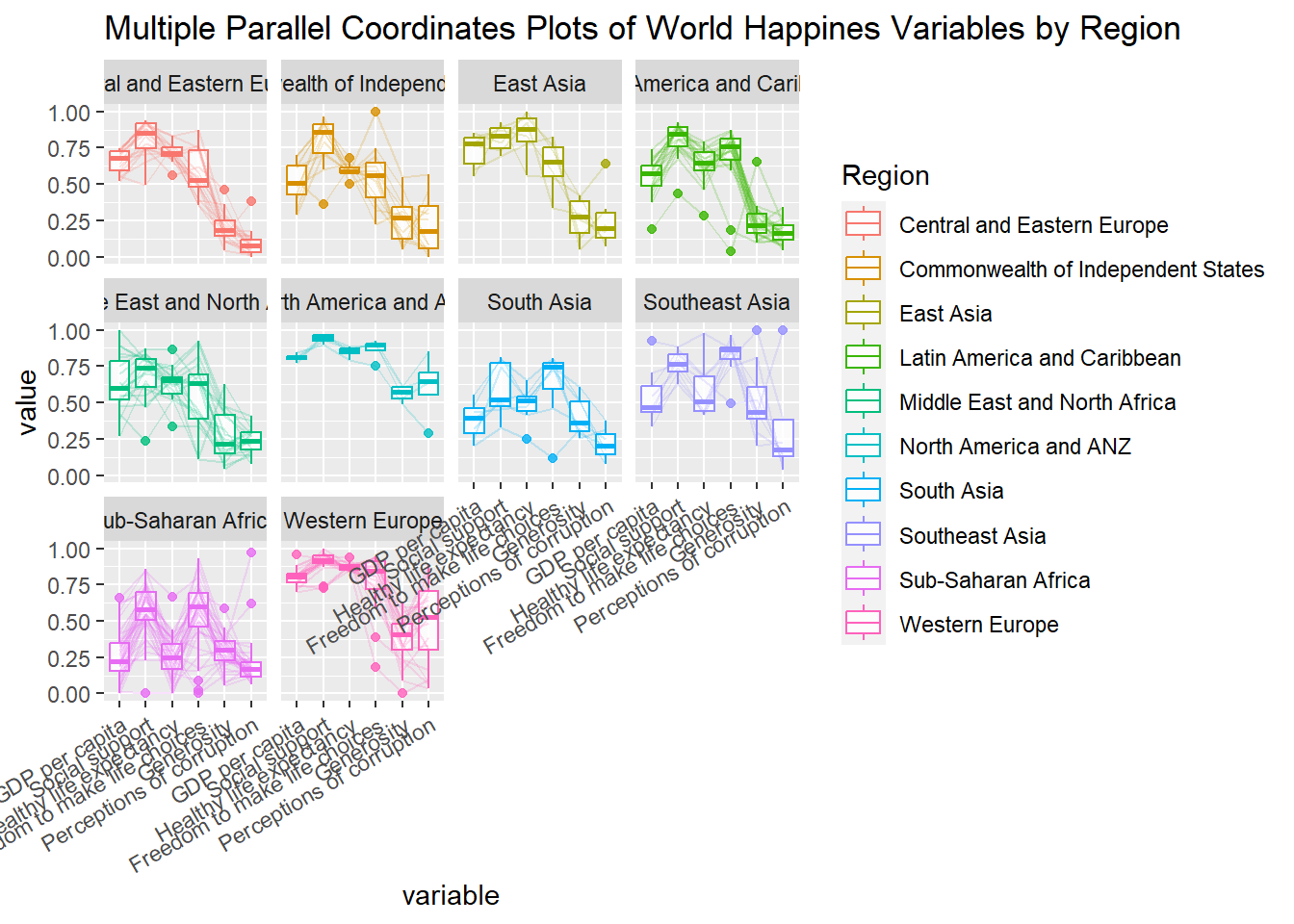

4. Plotting Interactive Parallel Coordinates Plot: parallelPlot methods

In this section, we will learn how to use functions provided in parallelPlot package to build interactive parallel coordinates plot.

4.1 The basic plot

The code chunk below plot an interactive parallel coordinates plot by using parallelPlot().

wh <- wh %>%
  select("Happiness score", c(7:12))
parallelPlot(wh,
             width = 320,
             height = 250)

When we click on any data point, the data from the same row is high lighted.

4.2 Changing the colour scheme

Let’s change the looks of the plot such as rotating the x-axis labels:

parallelPlot(wh,
             continuousCS = "YlOrRd",
             rotateTitle = TRUE)

4.3 Parallel coordinates plot with histogram

Similarly, we can add histograms on the chart to view the distributions.

histoVisibility <- rep(TRUE, ncol(wh))
parallelPlot(wh,
             rotateTitle = TRUE,
             histoVisibility = histoVisibility)

This comes to the end of this hands-on exercise. I have learned to make static and interactive parallel coordicates plots in R. Hope you enjoyed it, too!

See you in the next hands-on exercise 🥰